AMI SQL: Querying
This page covers AMI SQL query syntax for retrieving, joining, and analyzing data in AMI's in-memory database.
AMI SQL Introduction
AMI SQL is part of AMI's embedded scripting language AmiScript and provides SQL-like syntax for manipulating data from tables and other databases.
AMI SQL contains familiar syntax and instructions, providing a comprehensive instruction set for working with table(s) of data. Key features include:
- Retrieval: Accessing and Normalizing data from external sources.
- Blending: Joining and unioning on tables.
- Modifying: Inserting, Updating, and Deleting rows.
- Analyzing: Grouping, Sorting, and Filtering.
- Schema Definition: Creating, Updating, and Dropping tables.
Broadly speaking, the logic steps involved in data-visualization are:
-
Running a query, or set of queries, on external datasources and/or the AMI-Realtime database.
- Each datasource is predefined and uniquely named
- The results of queries on datasources will result in temporary, in-memory tables
- The queries can be constructed using user-input/user-selected/user-associated data
- In more advanced cases, the queries can be sequential, meaning the results from one query are then fed into a subsequent query (allowing for reactionary data blending)
-
Blending the results from Step 1, resulting in new temporary in-memory tables. 3. Building visualizations on the tables from Step 1 and/or Step 2.
Common SQL Queries Using AMI SQL
AMI SQL uses familiar syntax to other SQL systems, while also preserving Java-like qualities native to AmiScript. As a result, queries are generally more flexible than other SQL languages.
The following examples show common differences between AMI SQL and MySQL syntax:
-
==means equality:- AMI SQL:
SELECT * FROM Users WHERE userid == 15; - MYSQL:
SELECT * FROM Users WHERE userid = 15;
- AMI SQL:
-
Checking for null is done with equality, ex.
== null:- AMI SQL:
SELECT * FROM Users WHERE status == null; - MYSQL:
SELECT * FROM Users WHERE status IS NULL;
- AMI SQL:
-
Strings are surrounded in double quotes:
- AMI SQL:
SELECT * FROM Users WHERE name == "David"; - MYSQL:
SELECT * FROM Users WHERE name = 'David';
- AMI SQL:
-
"Matches" (
~~) instead of LIKE:- AMI SQL:
SELECT * FROM Users WHERE name ~~ "^Dav"; - MYSQL:
SELECT * FROM Users WHERE name LIKE 'Dav%';
(See Simplified Text Matching for pattern matching rules/expressions)
- AMI SQL:
-
Boolean expressions
&&works same as AND.||works same as OR:- AMI SQL:
SELECT * FROM Users WHERE userid == 15 AND status == null && name == "David"; - MYSQL:
SELECT * FROM Users WHERE userid = 15 AND status IS NULL AND name = 'David';
- AMI SQL:
-
By default all tables are
TEMPORARY, use thePUBLICkey word to make non-temporary tables:- AMI SQL:
CREATE TABLE MyTemporaryTable(id String); - MYSQL:
CREATE PUBLIC TABLE MyPermanantTable(id String);
- AMI SQL:
-
To return distinct values, equivalent to SQL
SELECT DISTINCT, useGROUP BYinstead:- AMI SQL:
SELECT name FROM User GROUP BY name - MYSQL:
SELECT DISTINCT name FROM User
- AMI SQL:
-
To return the number of distinct column values, use the AmiScript method
countUnique():- AMI SQL:
SELECT countUnique(name) AS unique_name_count FROM User - MYSQL:
SELECT COUNT(DISTINCT name) AS unique_name_count FROM User
- AMI SQL:
Query Clauses
SELECT
Overview
The SELECT clause is used to retrieve data from some underlying datasource, much like all standard SQL SELECT clauses.
In AmiScript, it can be used with a combination of the following options:
WHEREfor filteringORDER BYfor sortingGROUP BYfor aggregatingLIMITfor cropping
To tune results for individual tables.
Results can then be combined via unions (UNION) and/or joins (FROM ... JOIN ON). Complex Strings containing delimited data can be split into distinct rows via the UNPACK operation. Finally, see the CREATE TABLE AS clause for storing the final result of a select clause into another table.
To aggregate data, use the GROUP BY clause to identify any number of columns or derived values that should be used to group rows. Provide an alias (AS) for derived values to be used within the select clause. The select columns can only use aggregate functions (min, max, count, sum) on underlying rows and columns declared in the group-by clause.
To filter data, provide a WHERE clause which evaluates to a Boolean. True indicates don't filter. When filtering in conjunction with aggregating (GROUP BY), those records filtered out will not be considered for aggregation. To filter rows after aggregation, use the HAVING clause.
For projecting, supply columns to include in the SELECT clause. Derived values may be provided. Provide an alias (AS) for derived values or to rename a column. Use star (*) to include all columns or tblname.* to include only those columns from a particular table provided in the FROM clause.
To crop out rows, use the LIMIT clause. You may provide a number of rows to skip (offset) and a number of maximum rows to return (rowcount).
To sort, use the ORDER BY clause. If multiple expressions are given the left-most takes priority.
To union (concatenate) the results from multiple select clauses, use the UNION clause. The column names and types from the first select clause will provide the result set schema definition. If BYNAME is specified, then target columns and source columns are mapped by column name. If BYNAME is not specified all select clauses participating in a union must define the same number of columns. Note: this operates like a union all in many databases.
To join (blend) tables, supply all tables together in the FROM clause and a Cartesian product will be provided. For more advanced Joins, you can use a combination of the LEFT, RIGHT, OUTER, JOIN, ON and NEAREST clauses. See Joining Data section for details.
To process String columns containing multi-value delimited data, use the UNPACK col ON delimeter expression. This will split the string such that each entry will result in a new row.
Syntax
offset: Integer number of rows to skip.
rowcount: Integer number of maximum rows that will be returned.
Joining Data
Simple Cartesian Joins
Any number of tables can be joined by simply listing them after the FROM clause which will produce a Cartesian product, such that a row will be returned for each possible combination of rows from the source table. For example, the Cartesian product of a table with 5 rows and another table with 3 rows will produce 15 rows (5x3=15). Of course, the WHERE clause can be used to limit results to only the interesting combinations.
Handling Rows that don't match rows in other tables
For more granular control when joining two tables, use the JOIN syntax. There are 7 types of statements, let's assume two tables a and b:
- JOIN:
FROM a JOIN b ON expr: This is the same as FROM a,b WHEREexpr - LEFT JOIN:
FROM a LEFT JOIN b ON expr: A JOIN plus all records from table a that would otherwise be omitted (due to the expr). - LEFT ONLY JOIN:
FROM a LEFT ONLY JOIN b ON expr: Includes only records from table a that would otherwise be omitted (due to the expr). - RIGHT JOIN:
FROM a RIGHT JOIN b ON expr: A JOIN plus all records from table b that would otherwise be omitted (due to the expr). (Similar to LEFT JOIN, swapping a and b.) - RIGHT ONLY JOIN:
FROM a RIGHT ONLY JOIN b ON expr: Includes only records from table b that would otherwise be omitted (due to the expr). (Similar to LEFT ONLY JOIN, swapping a and b.) - OUTER JOIN: A JOIN plus all records from table
aand from tablebthat would otherwise be omitted (due to the expr). - OUTER ONLY JOIN: Includes only records from table a and from table b that would otherwise be omitted (due to the expr).
Joining to a nearest match
Use the NEAREST clause in conjunction with one of the above 7 JOIN clauses to match two records where there may not be an exact match, such as doing an "AsOf" join with timestamps. After the ON clause, include a NEAREST fuzzy_clause.
Consider: a JOIN b ON on_expr NEAREST fuzzy_clause, where the fuzzy clause is one of the 5 syntaxes:
a.cola == b.colb: For each row in tablea, join with the row in tablebthat satisfieson_exprand has the smallest delta betweencolaandcolb.a.cola <= b.colb: For each row in tablea, join with the row in tablebthat satisfieson_exprandcolais less than or equal tocolband has the smallest delta betweencolaandcolb.a.cola >= b.colb: For each row in tablea, join with the row in tablebthat satisfieson_exprandcolais greater than or equal tocolband has the smallest delta betweencolaandcolb.a.cola < b.colb: For each row in tablea, join with the row in tablebthat satisfieson_exprandcolais less than colb and has the smallest delta betweencolaandcolb.a.cola > b.colb: For each row in tablea, join with the row in tablebthat satisfieson_exprandcolais greater than colb and has the smallest delta betweencolaandcolb.
Note the ordering of table a vs b in the fuzzy_clause does not matter. For example b.colb >= a.cola is the same as a.cola <= b.colb.
General Examples
Nearest Join Examples
Assume two existing tables: Orders and MarketData.
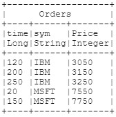
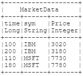
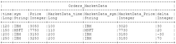
A JOIN will only include orders that have a satisfactory market data event. This example also calculates the price delta from the order vs the market.
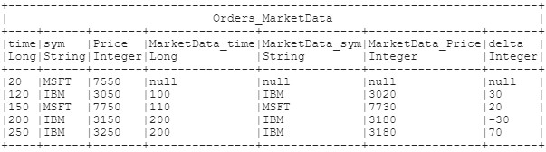
A LEFT JOIN will include all orders, event those without a market data event (using null as a place holder).
Join Examples
Let's assume you have two tables A and B, each with 1 column:
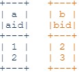
The value 1 only exists in the A table, the value 3 exists only in the B table and the value 2 existing in both tables. When comparing the data between them there are, exhaustively speaking, 7 different ways you could want to see what matches and what doesn't.
JOIN 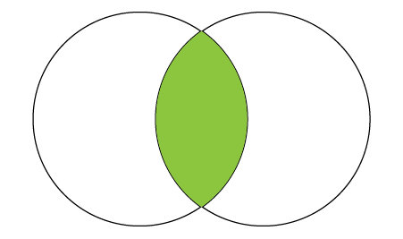 |
OUTER JOIN 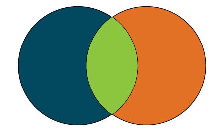 |
OUTER ONLY JOIN 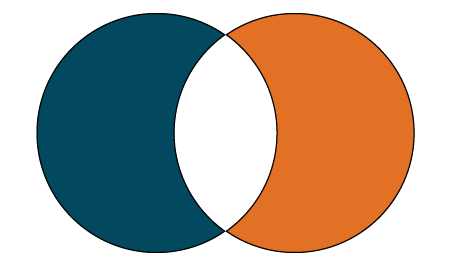 |
LEFT JOIN 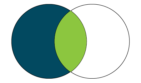 |
LEFT ONLY JOIN 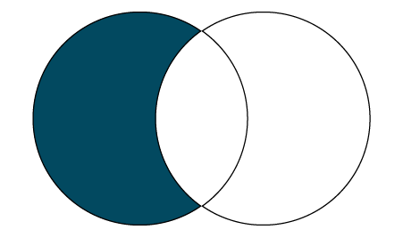 |
RIGHT JOIN 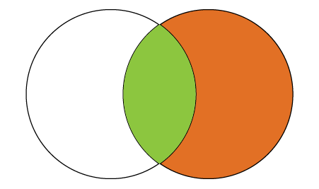 |
RIGHT ONLY JOIN 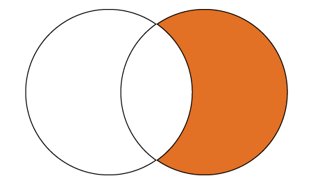 |
|
|---|---|---|---|---|---|---|---|
| Include Matches? | YES | YES | YES | YES | |||
| Includes Left W/O a Match on Right | YES | YES | YES | YES | |||
| Includes Right W/O a Match on Left | YES | YES | YES | YES |
JOIN Syntax: Return only those rows with values that coexist in both tables. (Note, this is the same as the natural join select * from a,b where a.aid==b.bid)

OUTER JOIN Syntax: Return all rows from both tables.
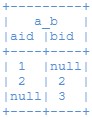
OUTER ONLY JOIN Syntax: Return rows in the left table that don't have matching rows in the right table and rows in the right table that don't have matching rows in the left table.
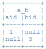
LEFT JOIN Syntax: Return all rows from the left table and only the rows in the right table matching rows in the left table.
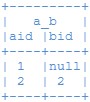
LEFT ONLY JOIN Syntax: Return only rows in the left table that don't have matching rows in the right table.

RIGHT JOIN Syntax: Return all rows from the right table and only the rows in the left table matching rows in the right table. (Note, this is equivalent to ... FROM b LEFT JOIN a ...)
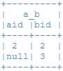
RIGHT ONLY JOIN Syntax: Return only rows in the right table that don't have matching rows in the left table. (Note, this is equivalent to ... FROM b LEFT ONLY JOIN a ...)

MULTIPLE TABLES INNER JOIN Syntax: Return rows that are joined based on columns from multiple tables. (AMI only supports inner join for mutliple table joins.)
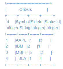
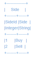
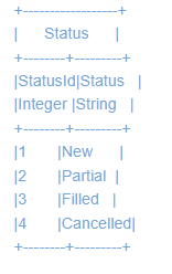
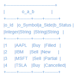
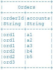
TABLE UNPACKING Syntax: Return the result unpacked by a specific delimiter based on a specific column.
ANALYZE
Overview
For cases where users want to perform rolling calculations and do not want to collapse rows of datas (which GROUP BY does), instead the AmiScript ANALYZE clause can be used to perform row-based calculations on a given table. This is loosely similar to SQL window functions.
In AMI, ANALYZE is used in conjunction with WINDOW to perform analysis (using AmiScript aggregate methods) on rows contained in a defined window, similar to a self-join.
Each window can define an order-by to allow for finer control over the order in which an aggregate is applied. Multiple windows may be defined. See window_expr for details.
When adding columns, the new cells will default to null. The column will be added to the end (right-most) of the table.
tblname: String name of the table to alter the schema of.
Example
PREPARE
Overview
This command allows the user to "prepare" additional columns whose values are calculated as aggregates across multiple rows. This is useful for calculations that require information from previous rows, for example a cumulative total.
There are a number of AmiScript Prepare functions that can be used inside the PREPARE clause to create columns with useful calculations. For example, for rolling totals, the STACK() can be used(see below).
Other useful options for a PREPARE clause include:
ORDER BY: In many cases, the ordering of rows in the input table is important, especially for running sums. TheORDER BYclause is useful to guarantee the correct ordering.PARTITION BY: Used to perform many aggregates on a single table, each aggregate considering only a subset of the table's rows based on some grouping criteria.
The general syntax is as follows:
tblname: String name of the table to alter the schema of.
Example: This example will produce the running total of stocks bought/sold and the amount spent.
Assigning Query Results to Local Variables
AMI Script supports the ability to execute queries and store the results into local variables. There are various ways the query results can be stored, beyond just Table objects, see type Coercion rules below.
This is the general form:
type var_name = query;
type: The type of local variable to store the query result.
var_name: Name of the local
query: A valid SQL query. Either select_clause, analyze_clause, or prepare_clause
Valid Type Coercion rules are listed below. Please note that an attempt to coerce the query result to an invalid type, will result in null.
List: Query results that have a single column can be stored to a List. Each value in the query result will be inserted into the list in order.
Set: Query results that have a single column can be stored to a Set. Each value in the query result will be inserted into the set in order, ignoring duplicate values (as per set's contract).
Map: Query results that have a single row can be stored to a map. The map's keys will be the columns' names, and the map's values will be the values of the first (and only) row.
Primitives: Queries that result in a single value (one row and one column) can be stored to a primitive variable. The value of the single cell is what will be stored.
Nested Expressions
alter_col_expr
colname: String name of the column to alter.
newname: String name of the column to create.
beforecol: String name of the existing column to add the new column before.
column_expr
colname: Name of the column that will contain results of expression.
* expands to available columns for all tables or specified table.
expr
See Standard Operators section.
forloop_expr
varname: Variable that can be referenced by expresions within the for loop.
start_const: Initial value of varname, inclusive.
end_const: Last number to loop over, inclusive unless the step would cause it to be skipped.
step: Positive number dictating size to increment or decrement varname by in each loop cycle.
A negative or zero step will cause an error. If start_const \<= end_const then step is used to increment, otherwise decrement.
in_expr
When only a single column will participate in the in clause:
When two or more columns will participate in the in clause:
The IN clause evaluates to true for a given row if the result of expr from the left hand expression exists in the right hand expression. If using multiple columns, the combination of the expr must match the combination of the values_expr or select_clause for a given row.
lambda_expr
The lambda expression allows for contained AmiScript to be executed once per row returned by the containing select statement. colname is the name of the column that the return value of this lambda will be placed in.
nested_select_expr
select_clause: Inner query to execute.
aliasname: Name of alias for use in column_expr and expr,
table_expr
*tblname: Name of table to include in select.
*aliasname: Name of alias for use in column_expr and expr.
type_expr
values_expr
where_expr
Expressions with the added IN clause (in_expr) funtionality
window_expr
window_name: The name of this window which is used in the preceding col_expr (in the analyze clause). For example, if the name of a window is "dates" then max(dates.open) would give you the max value of the open column for that window.
windowing_expr: The boolean expression that defines (for each row) the other rows that belong to the same window.
order_expr: Optional expression which determines the natural order of rows for the window. This is important for order dependent aggregates such as first(...) and last(...).
partitioning_expr: Optional expression which determines how the table is broken up before windowing is considered. In other words, two rows that evaluate to a different partitioning_expr will never belong to the same window.
prep_expr
stack(expr) |
running sum of expr from first to row n, inclusive |
count(expr) |
running count where expr!=null to the current row, inclusive |
norm(expr) |
similar to stack, but scaled so that the max value is one. Short hand for: stack(expr)/sum(expr). See dnorm(...) |
dnorm(expr) |
similar to stack, but scaled so that the min value is zero. Short hand for: (stack(expr) - expr)/sum(expr). This, in conjunction with norm(...) can used for preparing area charts that should fill an area, such as a pie chart. |
rank(expr) |
will evaluate expr for all rows and the lowest value will get 1, 2^nd^ will get 2, etc. If multiple rows expr evaluate to the same value, they will get the same ranking. |
urank(expr) |
will evaluate expr for all rows and the lowest value will get 1, 2^nd^ will get 2, etc. If multiple rows expr evaluate to the same value, the first occurrence gets the lower value. |
unique(expr) |
each unique evaluation of expr will return a unique integer, starting at 1. Repeat occurrences of expr will return the same integer value. |
offset(expr,offset) |
Will grab the value offset from the current row. If offset==0 use current row, negative number is nth prior row, positive number is nth future row. Evaluates to null if offset is out of bounds for current table. Ex: offset(price,-1) for first row returns null, for second row returns first row's price and for nth row returns (n-1)ths row's price |
kmeansCluster(expr1,expr2,...,nClusters,seed) |
Clusters data using the k-means clustering algorithm. Takes one or more expressions, followed by int nClusters specifying the number of clusters and long seed specifying the random seed for initializing the model parameters. The seed argument may be set to null if no specific seed is desired. Returns a column of integers labeling each record according to its learned cluster. Input expressions must evaluate to numbers. |
emGmmCluster(expr1,expr2,...,nClusters,seed) |
Same functionality as kmeansCluster(), but instead uses the expectation-maximization algorithm to train a Gaussian mixture model. |
viGmmCluster(expr1,expr2,...,nClusters,seed) |
Same functionality as kmeansCluster(), but instead uses the variational inference algorithm to train a Gaussian mixture model. |
agg_expr
sum(expr) |
Summation of all values, skips nulls . |
min(expr) |
Minimum value, skips nulls. |
max(expr) |
Maximum value, skips nulls. |
count(expr) |
Count of non-null values. |
countUnique(expr) |
Count of unique non-null values. |
cat(expr, delim, limit) |
Concatenates the first limit non-null values to a string with delim. Ex: cat(a,'/',2) selects the first 2 non-null values from column a and appends '/' at the end of each value. |
avg(expr) |
Average of all non-null values. |
var(expr) |
Population Variance of all non-null values. |
varS(expr) |
Sample Variance of all non-null values. |
stdev(expr) |
Population Standard Deviation of all non-null values. |
stdevS(expr) |
Sample Standard Deviation of all non-null values. |
first(expr) |
First value, may be null if first value is null. |
last(expr) |
Last value, may be null if last value is null. |
covar(expr1, expr2) |
Population Covariance of 1st expr and 2nd expr where both aren't null. |
covarS(expr1, expr2) |
Sample Covariance of 1st expr and 2nd expr where both aren't null. |
cor(expr1, expr2) |
Correlation of 1st expr and 2nd expr where both aren't null. Returns 0 - 1. |
beta(expr1, expr2) |
Beta of 1st expr and 2nd expr where both are not null. The beta function is defined as beta(x, y) = covar(x, y) / var(y). If stdev(y) = 0, the expression returns NaN. |
avgExp(expr, decay, desc) |
The exponentially weighted average of non-null values with a specified decay rate. Desc of true/false means first/last row are highest weighted. |
avgGauss(expr, variance) |
The Gaussian weighted average of non-null values, such that the middle value has highest weight. |
median(expr) |
The median of all non-null values. |
percentileCont(expr) |
Returns the value at the percentile provided. Is interpolated and might not be equal to any value within the supplied dataset. |
percentileDisc(expr) |
Returns the value nearest to the percentile provided. |